Spatial Performance Assessment for Cognitive Evaluation
I am working on a wide range of topics involving human motion at all scales. As a spatial data scientist, I bring together Computer Science, Cognitive Science and Spatial Sciences.
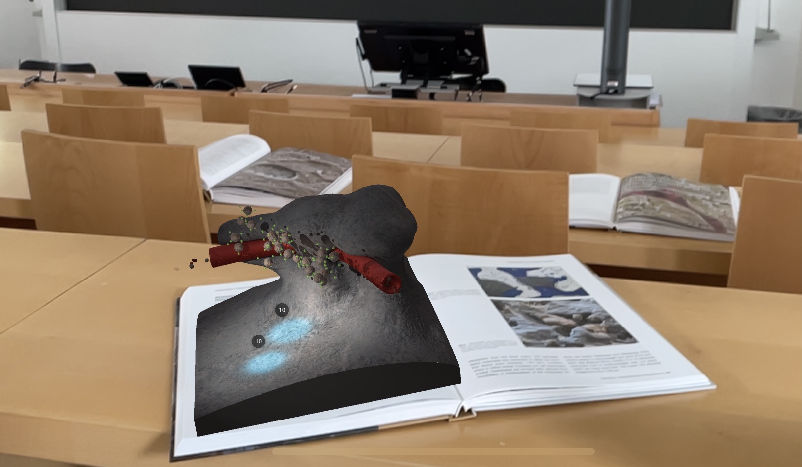
I ended up as an academic but this week I am happy to announce my newest paper as a first author in JMIR Publications Serious Games on a learning game I created together with the ETH Game Technology Center, University of Zurich, and Medical University of Vienna with support from Quintessence Publishing Deutschland. Our Game…
Last year during my first steps as a postdoc I applied to the institutional Swiss Open Research Data Grants. For my work at the Center for Sustainable Future Mobility (CSFM) at ETH Zürich, I gained the support of Prof. Kay W. Axhausen and Prof. Martin Raubal to submit a project together with the Swiss Data…
This is a question that recently haunted me. Previously, at the Game Technology Center (GTC) at ETH Zürich, I was privileged enough to sit on a deployed pipeline. It creaks sometimes but in general, it works well. For a new project with Future Health Technologies at the Singapore ETH Center, there was no such luck.…